Generative Adversarial Networks (GANs) are a type of deep neural network architecture used for generating new data samples that are similar to a given dataset. GANs consist of two neural networks, a generator and a discriminator, which are trained in an adversarial manner. GANs were introduced by Ian Goodfellow and his colleagues in 2014, and have since become one of the most popular and powerful tools for generating realistic synthetic data. The generator generates new data samples, while the discriminator tries to distinguish between real and fake data samples. As the generator improves, the discriminator becomes better at distinguishing real from fake samples, leading to a feedback loop that drives the generator to produce more realistic samples.

GANs have a wide range of applications, including image synthesis, data augmentation, and anomaly detection. In this blog, we will explore how GANs work and provide some code examples to illustrate their usage.

Architecture of GANs

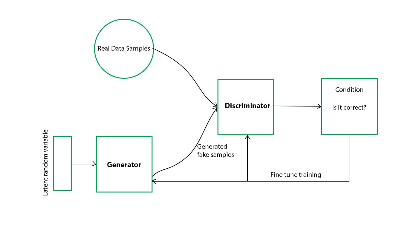
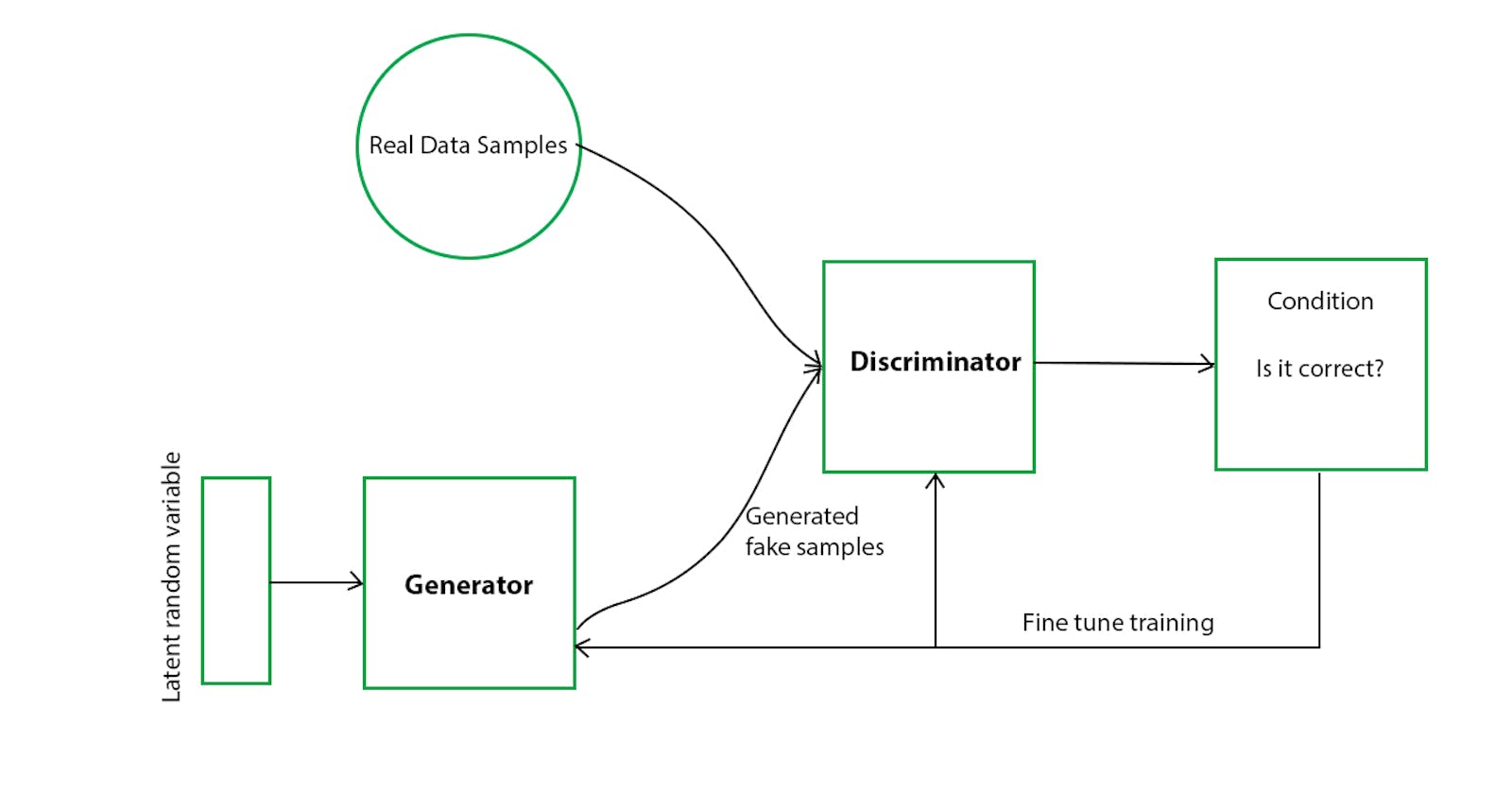
How GANs Work

GANs consist of two neural networks, a generator, and a discriminator. The generator takes a random noise vector as input and generates a new data sample, while the discriminator takes a data sample as input and outputs a binary classification label indicating whether the sample is real or fake. The goal of the generator is to generate samples that are realistic enough to fool the discriminator, while the goal of the discriminator is to distinguish between real and fake samples.

The training process for GANs is done in an adversarial manner. The generator and discriminator are trained in alternating epochs, with the generator trying to generate samples that fool the discriminator and the discriminator trying to correctly classify real and fake samples. The loss function for GANs is a minimax game, where the generator tries to minimize the probability that the discriminator correctly classifies fake samples, and the discriminator tries to maximize the probability that it correctly classifies real and fake samples.

Code Example

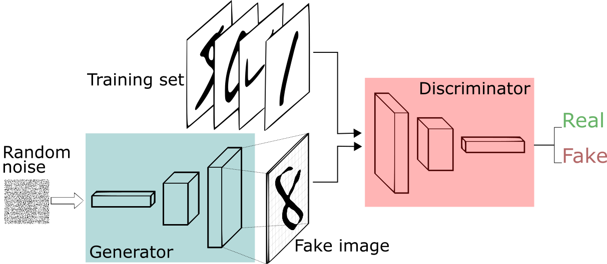
Now, let's see how to implement a simple GAN using PyTorch. In this example, we will generate new images that look like handwritten digits from the MNIST dataset.

import torch
import torch.nn as nn
import torch.optim as optim
import torchvision
import torchvision.transforms as transforms
import numpy as np
import matplotlib.pyplot as plt

# Set random seed for reproducibility
np.random.seed(42)
torch.manual_seed(42)

# Load MNIST dataset
transform = transforms.Compose(
    [transforms.ToTensor(),
     transforms.Normalize((0.5,), (0.5,))])

trainset = torchvision.datasets.MNIST(root='./data', train=True,
                                        download=True, transform=transform)
trainloader = torch.utils.data.DataLoader(trainset, batch_size=128,
                                          shuffle=True, num_workers=2)

# Define generator network
class Generator(nn.Module):
    def __init__(self, input_size=100, output_size=784):
        super(Generator, self).__init__()
        self.fc1 = nn.Linear(input_size, 128)
        self.fc2 = nn.Linear(128, 256)
        self.fc3 = nn.Linear(256, output_size)
        self.relu = nn.ReLU()
        self.tanh = nn.Tanh()

    def forward(self, x):
        x = self.relu(self.fc1(x))
        x = self.relu(self.fc2(x))
        x = self.tanh(self.fc3(x))
        return x

# Define discriminator network
class Discriminator(nn.Module):
    def __init__(self, input_size=784, output_size=1):
        super(Discriminator, self).__init__()
        self.fc1 = nn.Linear(input_size, 256)
        self.fc2 = nn.Linear(256, 128)
        self.fc3 = nn.Linear(128, output_size)
        self.relu = nn.LeakyReLU(0.2)
        self.sigmoid = nn.Sigmoid()

    def forward(self, x):
        x = self.relu(self.fc1(x))
        x = self.relu(self.fc2(x))
        x = self.sigmoid(self.fc3(x))
        return x

# Instantiate generator and discriminator networks
generator = Generator()
discriminator = Discriminator()

# Define loss function and optimizer
criterion = nn.BCELoss()
gen_optimizer = optim.Adam(generator.parameters(), lr=0.0002, betas=(0.5, 0.999))
disc_optimizer = optim.Adam(discriminator.parameters(), lr=0.0002, betas=(0.5, 0.999))

# Define number of epochs and size of noise vector
num_epochs = 100
noise_size = 100

# Train GAN
for epoch in range(num_epochs):
    for i, data in enumerate(trainloader, 0):
        # Train discriminator on real data
        discriminator.zero_grad()
        real_data = data[0].view(-1, 784)
        real_labels = torch.ones(real_data.size(0), 1)
        real_outputs = discriminator(real_data)
        real_loss = criterion(real_outputs, real_labels)
        real_loss.backward()

        # Train discriminator on fake data
        noise = torch.randn(real_data.size(0), noise_size)
        fake_data = generator(noise)
        fake_labels = torch.zeros(fake_data.size(0), 1)
        fake_outputs = discriminator(fake_data.detach())
        fake_loss = criterion(fake_outputs, fake_labels)
        fake_loss.backward()

        disc_optimizer.step()

        # Train generator
        generator.zero_grad()
        noise = torch.randn(real_data.size(0), noise_size)
        fake_data = generator(noise)
        fake_labels = torch.ones(fake_data.size(0), 1)
        fake_outputs = discriminator(fake_data)
        gen_loss = criterion(fake_outputs, fake_labels)
        gen_loss.backward()
        gen_optimizer.step()

        # Print training progress
        print('[%d/%d] Discriminator Loss: %.3f, Generator Loss: %.3f' %(epoch+1, num_epochs, (real_loss+fake_loss).item(), gen_loss.item()))

# Generate and visualize some sample images
num_samples = 16
noise = torch.randn(num_samples, noise_size)
generated_data = generator(noise).detach().numpy()

fig, axs = plt.subplots(4, 4, figsize=(4,4))
axs = axs.flatten()

for i in range(num_samples):
    img = generated_data[i].reshape(28, 28)
    axs[i].imshow(img, cmap='gray')
    axs[i].axis('off')

plt.show()

"""
Note that this code is designed to be run in a Jupyter notebook or in a Python script, and assumes that PyTorch, NumPy, and Matplotlib have been installed. To run the code, simply copy and paste it into a Python environment and execute it. The code will download the MNIST dataset, train the GAN, and generate a grid of sample images.
"""

Code Implementation diagram:

Training Process of GAN:

The training process for GANs involves iterating between training the generator and training the discriminator, to achieve a Nash equilibrium, where the generator produces data that is indistinguishable from the real data, and the discriminator is unable to differentiate between the real and fake data. This equilibrium is often referred to as the "minimax" solution, as both networks are trying to minimize their respective loss functions while simultaneously trying to maximize the other network's loss.

Discussing pros, cons, and also its future scope:

One of the main advantages of GANs is their ability to generate high-quality, diverse samples that capture the underlying distribution of real data. GANs have been used to generate images, videos, music, and even text. Some examples of applications of GANs include generating realistic images of faces, creating photorealistic landscapes, and generating new molecules for drug discovery.

In addition to their practical applications, GANs have also been the subject of extensive research and development, with many different variations and extensions proposed over the years. Some of the most popular GAN variants include Conditional GANs (cGANs), which allow for the generation of data based on specific conditions, and CycleGANs, which enable the generation of data from one domain to another.

In terms of challenges and limitations, GANs can be difficult to train and can suffer from instability, mode collapse, and other issues. They also require a large amount of data and computational resources to train effectively. However, despite these challenges, GANs remain one of the most exciting and promising areas of machine learning research today.

Conclusion

In conclusion, Generative Adversarial Networks (GANs) have emerged as one of the most powerful and versatile tools in the field of machine learning. By training a generator network to produce realistic-looking data that can fool a discriminator network, GANs have the ability to generate high-quality synthetic data that can be used for a variety of purposes, including image and video synthesis, text generation, and more.

While GANs are not without their challenges and limitations, they continue to be the subject of intense research and development, with new variations and extensions being proposed all the time. As the field of machine learning continues to evolve, it seems likely that GANs will remain an important area of study, with potential applications in everything from entertainment and art to medicine and science.

Overall, GANs represent a fascinating intersection of creativity and technology and are sure to remain a topic of interest for researchers and enthusiasts alike.

Thank you for reading this blog. :)